我们已经对White Noise有了比较全面的了解,也已经能对White Noise做一些简单的应用了,但是White Noise的缺点还是很明显的,比如:像素点间的过渡过于生硬,无法产生平滑的过渡效果。这也是我们引入Value Noise的原因。
#define STEP 200.

float hash(float x) {
	return fract(sin(x * 13452.) * 1000.);
}

float hash2(vec2 v) {
	return fract(sin(dot(v, vec2(64.24232, 87.873)))*10232.);
}

float hash3(vec3 v) {
	return fract(sin(dot(v, vec3(64.24232, 87.873, 76.635)))*10232.);
}

float valueNoise(vec2 v) {
	vec2 f = floor(v);
    vec2 r = smoothstep(vec2(0.), vec2(1.), fract(v));

    float lb = hash2(f);
    float rb = hash2(f+vec2(1.,0.));
    float lt = hash2(f+vec2(0.,1.));
    float rt = hash2(f+vec2(1.,1.));

    float b_line = mix(lb, rb, r.x);
    float t_line = mix(lt, rt, r.x);

    return mix(b_line, t_line, r.y);
}

float valueNoise3(vec3 v) {
	vec3 f = floor(v);
    vec3 r = smoothstep(vec3(0.), vec3(1.), fract(v));

    return mix(
    	mix(mix(hash3(f), hash3(f+vec3(1.,0.,0.)), r.x),
            mix(hash3(f + vec3(0.,1.,0.)), hash3(f + vec3(1.,1.,0.)), r.x),
            r.y),
        mix(mix(hash3(f+vec3(0.,0.,1.)), hash3(f+vec3(1.,0.,1.)), r.x),
            mix(hash3(f + vec3(0.,1.,1.)), hash3(f + vec3(1.,1.,1.)), r.x),
            r.y),
        r.z
    );
}

float sphere(vec3 p) {
    // p.x += dot(p.yz, p.yz);
    // p.z -= dot(p.xy, p.xy) * cos(iTime);
    float fireK = smoothstep(0.9,.5,valueNoise3(p*10.+iTime*3.));
    // vec3 fire = mix(vec3(1.,0.,0.), vec3(1., 1., 1.), fireK);
    p.y -=  fireK;
	return length(p) - 1.;
}

vec2 dist(vec3 p) {
    vec2 sphereDist = vec2(sphere(p-vec3(0., 0., 0.)), 2.);
	vec2 tableDist = vec2(p.y + 1., 1.);
    return tableDist.x < sphereDist.x?tableDist:sphereDist;
}

vec3 calNormal(vec3 p) {
	vec2 k = vec2(0.001, 0.);
    return normalize(vec3(
    	dist(p + k.xyy).x - dist(p - k.xyy).x,
        dist(p + k.yxy).x - dist(p - k.yxy).x,
        dist(p + k.yyx).x - dist(p - k.yyx).x
    ));
}

vec2 raymarch(vec3 ro, vec3 rd) {
    float t = 0.;
    float y = -1.;
    for(float i = 0.; i<STEP; i++) {
    	vec2 d = dist(ro + rd*t);
        if(d.x < .001) {
            y = d.y;
        	break;
        }
        if(t > STEP) {
            t = -1.;
            break;
        }
        t += d.x;
    }
    return vec2(t, y);
}

void mainImage( out vec4 fragColor, in vec2 fragCoord )
{
    // Normalized pixel coordinates (from -1 to 1)
    vec2 uv = 2. * (fragCoord - 0.5*iResolution.xy) / iResolution.y;

    // Time varying pixel color
    vec3 skyCol = vec3(0.2, 0.6, 1.) - 0.3 * uv.y;
	vec3 col = skyCol;
    vec3 ro = vec3(0.,0.,3.);
    vec3 rd = normalize(vec3(uv.xy, -1.));
    vec2 t = raymarch(ro, rd);
    if(t.x > 0.) {
        vec3 mate = vec3(0.2);
        vec3 sunCol = vec3(1.);
        vec3 p = ro + rd*t.x;
        vec3 n = calNormal(p);
        vec3 sunDir = normalize(vec3(0.8,0.4,0.2));
        float sunDiff = max(0., dot(n, sunDir));
        float skyDiff = clamp(0.5 + 0.5*dot(vec3(0.,1.,0.), n), 0., 1.);
    	float sunShadow = step(raymarch(p + n*0.01, sunDir).x, 0.);

        col = mate * vec3(8.0,5.0,3.0) * sunDiff * sunShadow;
        col += mate * skyDiff * vec3(0.2, 0.6, 1.);
        if(t.y > 1.) {
            float fireK = smoothstep(0.2,.5,valueNoise3(p*10.+iTime*3.));
            vec3 fire = mix(vec3(1.), vec3(1., 0.5, 1.), fireK);
        	col *= fire;
        } else {
        	// col += hash(uv.y);
        }
    }
    col = pow(col, vec3(0.4545));
    // Output to screen
    fragColor = vec4(col,1.0);
}
上面代码是本篇实验的实践结果,具体做法需要结合Raymarching部分进行讲解,完整代码后续在Shader实验室: RayMarching(二)中进行详细分析。我们对Noise的拆解还是按照从1D到3D的步骤进行描述。
1D Value Noise
在开篇部分我们说过Value Noise与White Noise的区别是像素点的过渡是否平滑,而要实现平滑过渡很直观的想法是通过线性插值来进行处理,而线性插值的前提是:必须是两个不同的值才可实现插值。根据推论,我们可取floor(x)与floor(x)+1.0作为数据源,再结合随机与噪声:White Noise篇中推出的随机算法进行计算,形如:
float random(float x) {
     return fract(sin(x * 457.87) * 10000.0);
}
y1 = floor(x);
y2 = floor(x)+1.0;
// 以下为伪代码,?号为未知数值, 代表如何插值还未知
float res = mix(random(y1), random(y2), ?);
上述代码如何进行插值是我们接下来要讨论的重点,我们可结合mix函数的定义来分析(等同于Cg中的lerp函数)。
// 当w为0时,返回a,当w为1时返回b,否则返回a与b的插值
float mix(float a, float b, float w) {
   return a + w*(b-a);
}
根据mix的定义可知,mix函数的第三个参数最好是一个0~1间的数,分析到这,我们可以很清晰的想到可以使用fract(x)作为mix函数的第三个参数,原因可看Shader实验室:fract函数。我们把fract(x)代入:
float res = mix(random(y1), random(y2), fract(x));
效果如下:
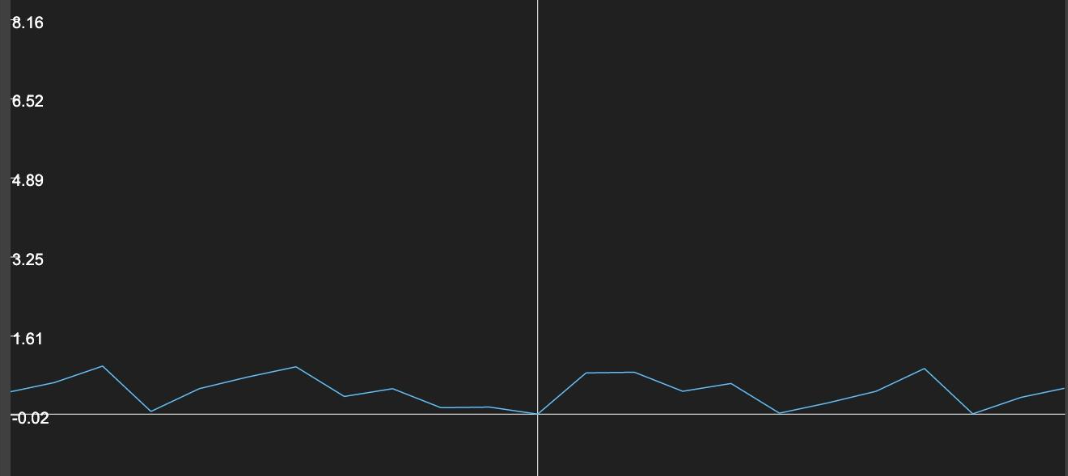
生成结果发现线与线间的连接处很生硬,如何让其更平滑?或者我们分析过的函数中,哪个函数可以做到平滑?是的,smoothstep函数,那就上吧:
float res = mix(random(y1), random(y2), smoothstep(0., 1., fract(x)));
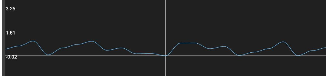
好了,掌握了1D Value Noise的生成,一起分析下2D Value Noise吧。
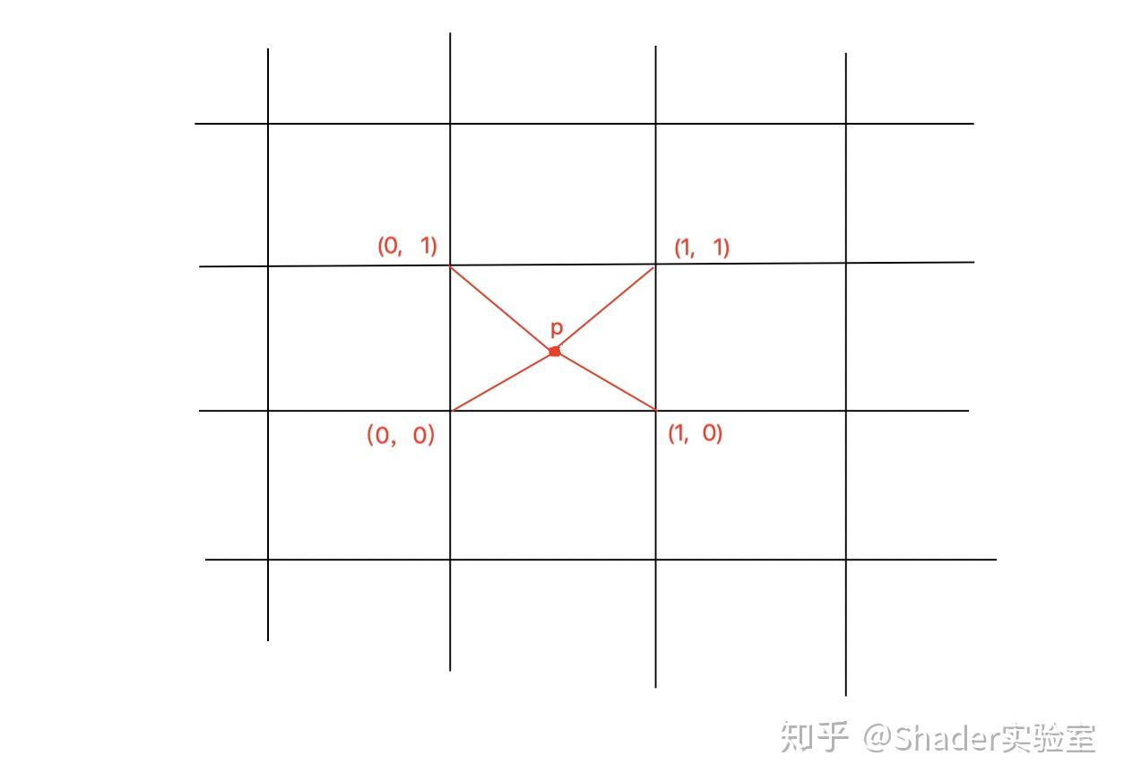
2D Value Noise
2D Value Noise与1D Value Noise的原理类似,区别在于2D Value Noise在平面上做插值,如图:
在代码实现上,可通过下图所示方式:
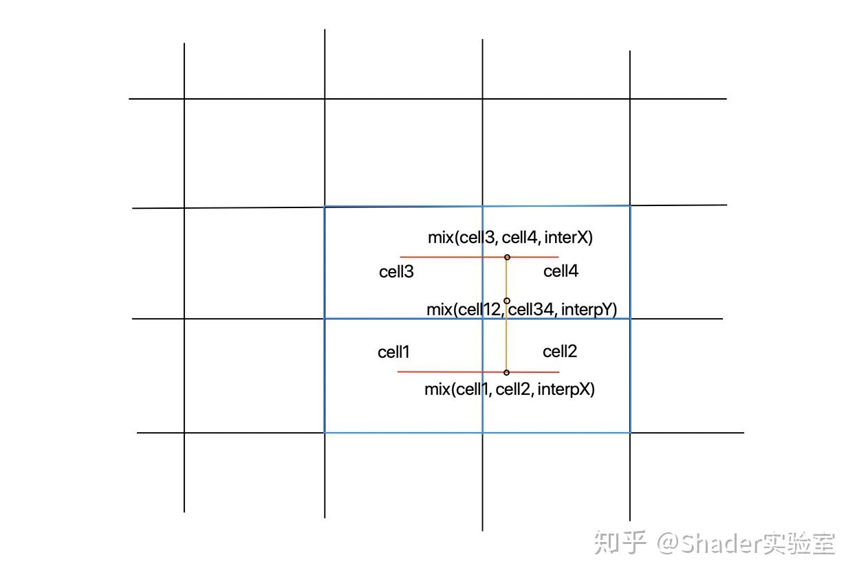
示意代码如下:
vec2 f = floor(vec2(x, y));
vec2 i = fract(vec2(x, y));
float ceil1 = random(f);
float ceil2 = random(f+vec2(1,0));
float ceil3 = random(f+vec2(0,1));
float ceil4 = random(f+vec2(1,1));
float ceil12 = mix(ceil1, ceil2, smoothstep(0, 1, i.x));
float ceil34 = mix(ceil3, ceil4, smoothstep(0, 1, i.x));
float result = mix(ceil12, ceil34, i.y);
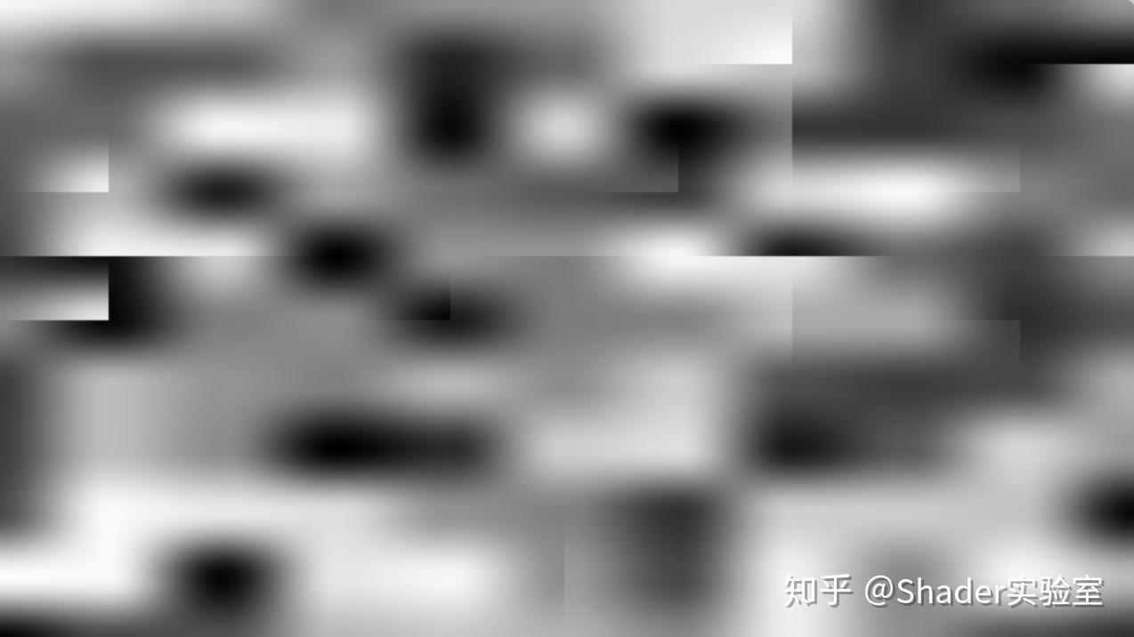
2D Value Noise的输出结果如下:
3D Value Noise
3D Value Noise相比2D Value Noise多了一个维度,但是不管是1D Value Noise 还是 2D Value Noise,还是我们现在要分析的3D Value Noise原理都是一样的,3D Value Noise的原理如下:
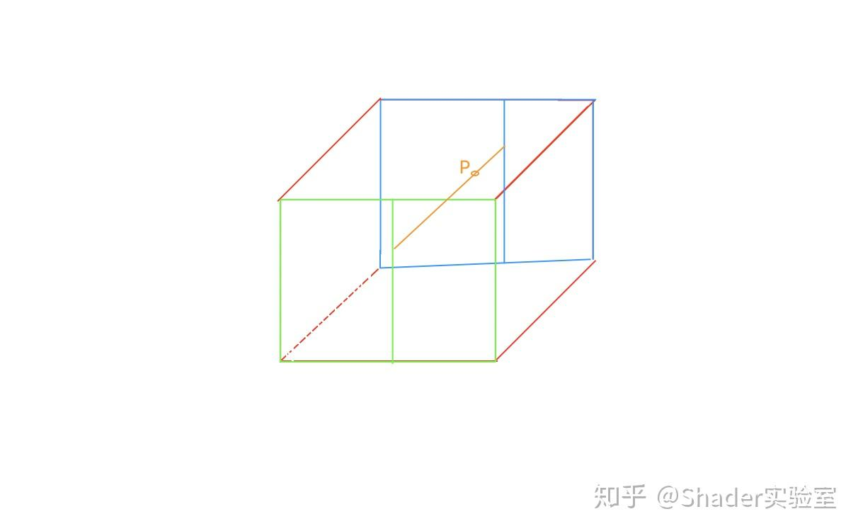
上图是3D立方体,其中绿色线框与蓝色线框分别为立方体的前面与背面,绿色线框与蓝色线框部分的Value Noise值可通过2D Value Noise的插值方式求取,最后通过mix( cell(green), cell(blue), smoothstep(0, 1, fract(z)))求得;示例代码如下:
float valueNoise3(vec3 v) {
     vec3 f = floor(v);
     vec3 r = smoothstep(vec3(0.), vec3(1.), fract(v));
     return mix(
         mix(mix(random(f), random(f+vec3(1.,0.,0.)), r.x),
              mix(random(f + vec3(0.,1.,0.)), random(f + vec3(1.,1.,0.)), r.x),
              r.y),
         mix(mix(random(f+vec3(0.,0.,1.)), random(f+vec3(1.,0.,1.)), r.x),
              mix(random(f + vec3(0.,1.,1.)), random(f + vec3(1.,1.,1.)), r.x),
              r.y),
         r.z
     );
}
Value Noise部分就到这里啦,感兴趣的伙伴可自己实现开篇的案例,由于Value Noise实现的效果会有块状的效果产生(可查看2D Value Noise的输出图片),这也是Perlin Noise提出的原因。
感兴趣的伙伴可扫描下方二维码关注我们吧